Working with visual data (images, videos) and its metadata is no picnic . Especially if you are running analytics on them. You not only need to deal with the visual data itself, but also have to deal with multimodal metadata (i.e., bounding boxes coordinates and their labels, or a text description with the content of the image), and even feature vectors, just to name a few. When you complete a project and attempt to apply a "cookie-cutter" approach to solve a new, yet similar business problem, you discover that you have to deal with various types of metadata all over again. There is not much re-use. Your prior experience does help, but only linearly, not exponentially. If you were wondering what is missing, you are not alone.
If you have trained an ML model to run object detection, segmentation, or tracking, you are familiar with the long list of steps needed before you even start tuning your neural network model's parameters (let alone run the training and wait for the results).
Let’s walk through some of the steps. For this, let’s use as an example a popular dataset: Common Objects in Context (or COCO for short). COCO is a large-scale object detection, segmentation, and captioning dataset that includes more than 200 thousand images, together with annotations. These annotations include bounding boxes, object segmentation, and recognition in context for about 1.5 million different objects. While COCO could be stored on a single machine (less than 100GB, including images and labels, bounding boxes, and segmentation information), its rich annotations and complexity, make it a great example dataset to start with.
COCO can be used for training models on general objects (for which labels are provided) to later train (using transfer learning) on more specific objects based on application specific needs. You could also select a subset of the images for training, throwing away images that are not relevant to your application (i.e., images containing objects and labels that are no relevant).
Now, consider a ML developer constructing a pipeline for object detection . First, you have to have all images in an accessible place, and the right data structures that associate each image and its bounding boxes with the right labels. This requires assigning consistent identifiers for the images and adding their metadata in some form of relational or key-value database. Finally, if the ML pipeline needs images that are of a size different than the original ones present in the dataset, there is additional compute diverted towards pre-processing after the images are fetched. All these steps require integration of different software solutions that provide various functionalities that can then be stitched together with a script for this specific use case.
More generally, data scientists and machine learning developers usually end up building an ad-hoc solution that results in a combination of databases and file systems to store metadata and visual data (images, videos), respectively. There are N technologies for dealing with visual data and M technologies for metadata. Each is mostly unaware of each other, therefore a connector, or a "glue", has to be written in order to have a solution for a given problem, as we describe in greater detail here . Companies (or team within the same company) select one of each technology according to immediate needs, which results in multiple implementations for each of N*M connectors. These ad-hoc solutions make replicating experiments difficult, and more importantly, they do not scale well when deployed in the real-world. The reason behind such complexity is the lack of a one-system that can be used to store and access all the data the application needs.
Now, to add more real-world complexity, less assume we work in a team of ML engineers and data scientist. There are many steps in the ML pipeline, and many people involved in the task. It is important for the team to share data, intermediate results, and good practices, and, given usually growing scale, having multiple replicas of the dataset is no longer an option. An ad-hoc solution with loosely defined interfaces is painful to maintain and error-prone. What we need is a database system design for visual data and ML workloads.
The good news is that at ApertureData, we have been focusing all our efforts on solving these problems. Our solution, ApertureDB , provides an API that enables a smooth interaction with visual data. Images, videos, bounding boxes, feature vectors and labels are first-class entities.
Accelerating Data Preparation
Let’s see how easy it is to interact with the COCO dataset with ApertureDB in Python. As a starting point, we have pre-populated the dataset on ApertureDB. Connecting to ApertureDB is very simple. All we need to do is instantiate a connector to the database, using the binary-compatible VDMS connector (VDMS is the original and open-source version of ApertureDB):
import vdms
db = vdms.vdms() # Instanciate a DB connector
db.connect(“coco.datasets.aperturedata.io”)
Now, with a connection open to the database, we can start sending queries. We can do this in two ways: using the Native API , or using ApertureDB Object Model API. The latter allows us to interact with the data in the database as if we were dealing with Python Objects, and without the need to write query using the native API. We will use the Object Model API for this demonstration.
Here is an example of how easy it is to filter and retrieve images. Let’s retrieve only the images that are larger than 600x600 pixels, and we only one images of a specific type of Creative Common License:
from aperturedb import Image
imgs = Image.Images(db)
const = Image.Constraints()
const.greater(“width”, 600)
const.greater(“height”, 600)
const.equal("license", 4)
imgs.search(constraints=const)
And that’s it. The imgs object will contain a handler for all the images. we can pass those images to our favourite framework for processing (Pytorch, Tensorflow, etc). We also provide tools for quick visualization. Showing the images is as simple as it can be:
imgs.display(limit=6) # We limit the number of images for display purposes.
Combining the snippets above will help us find the images that are 600x600 in resolution and covered by license 4 with a few (6) examples displayed below:

Even if the images are now fully accessible to the application and ready for use, they will be expected to be preprocessed with basic operations like a resize (to make it the size expected in the input layer of our neural network), or even a normalization step. It is a shame that we tranferred the full-size image from ApertureDB only to later discard most of that information with a resize (which most likely will downsample the image to, say, 224x224). But because ApertureDB was designed with ML use cases in mind, these basic pre-processing operations are supported as part of the API. Instead of retrieving the full-size images, we can simply indicate that we want the images to be resize before retrieving them, saving bandwidth and accelerating the fetching significantly.
We can retrieve resized images directly (and even rotate them as a data augmentation technique) by simply doing:
import vdms
from aperturedb import Image
db = vdms.vdms()
db.connect("coco.datasets.aperturedata.io")
imgs = Image.Images(db)
const = Image.Constraints()
const.greater("width", 600)
const.greater("height", 600)
ops = Image.Operations()
ops.resize(224, 224)
ops.rotate(45.0, True)
imgs.search(constraints=const, operations=ops)
imgs.display(limit=6)
The result is:

As part of our pipeline, we may also need to retrieve metadata associated with the images. We can easily obtain a list of all the metadata properties associated with the images by doing:
prop_names = imgs.get_props_names()
print(prop_names)
# Reponse:
['aspect_ratio', 'coco_url', 'date_captured', 'date_insertion', 'file_name', 'flickr_url', 'height', 'id', 'license', 'seg_id', 'type', 'width', 'yfcc_id']
For instance, let’s retrieve the metadata information associated with the images we retrieved in our last query:
import json
props = imgs.get_properties(["coco_url", "height", "width"])
print("Response: ", json.dumps (props, indent=4))
Response:
{
"341010": # This is the image id
{
"coco_url": "http://images.cocodataset.org/train2017/000000341010.jpg",
"height": 640,
"width": 640
},
"208867": # This is the image id
{
"coco_url": "http://images.cocodataset.org/train2017/000000208867.jpg",
"height": 640,
"width": 628
},
…
}
What about bounding boxes and segmentation masks?
Because ApertureDB recognizes images, videos, and bounding boxes as first-class citizens of the database, we can easily retrieve and show these objects with little effort. For instance, retrieving the bounding boxes associated with the images is as simple as doing:
imgs.display(limit=6, show_bboxes=True)
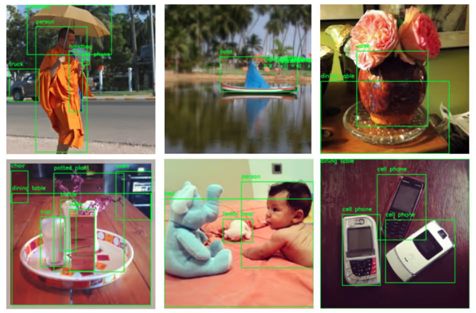
Similarly, let’s retrieve the segmentation annotations associated with the images. Same as bounding boxes, we can do that with a simple function parameter, as follows.
imgs.display(limit=6, show_segmentation=True)

Note that the segmentation masks needed will be retrieved from the ApertureDB only when explicitly requested (in this case, for displaying them). You can also use other interfaces to retrieve bounding boxes coordinates, labels, and segmentation polygons directly as JSON objects or Python dictionaries.
Support for Similarity Search
Another important piece of the puzzle when dealing with visual data are feature vectors. For instance, in the context of the COCO dataset, feature vectors represent information about the nature or content of the images. Feature vectors represent this information in a high-dimensional hyper-space, which can be used to perform a “similarity search” (i.e., finding objects that are similar). This similarity is not tied to metadata (like labels or image properties), but rather to “how similar” those feature vectors are. Because ApertureDB recognizes feature vectors as part of its interface, associating feature vectors to images, and, later, searching for similar images is as simple as it can be.
Let's take as an example the following image:
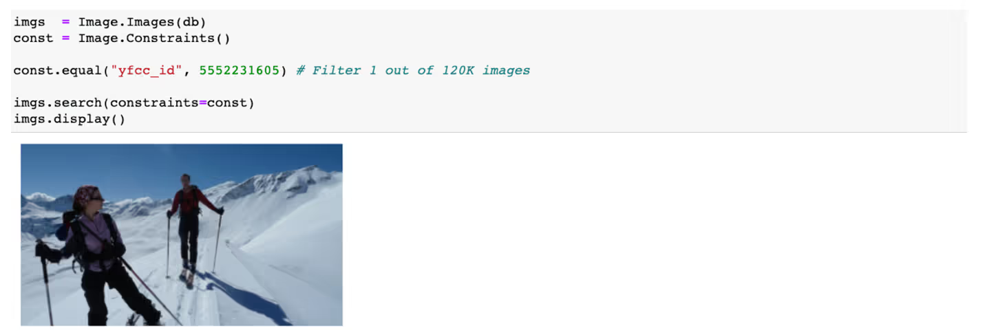
Now, let’s find the 6 most similar images (and, their bounding boxes, just because it is so easy):
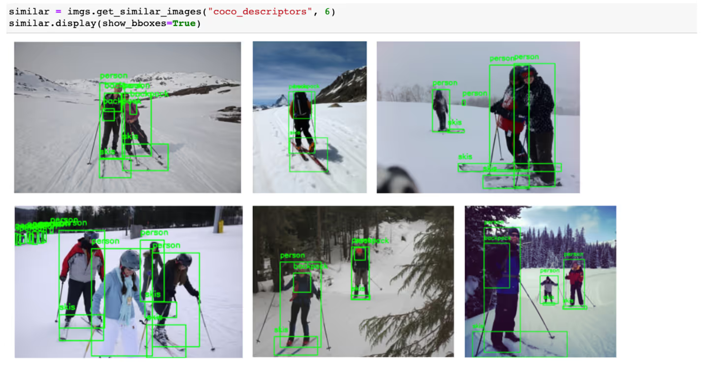
As we have seen, interacting with visual data has never been easier, and we are only scratching the surface of ApertureDB’s powerful API.
Last, but not least, ApertureDB offers a web user interface that allows user to explore the content of the database and run image search. Here is an example of what our webUI looks like for the COCO dataset:
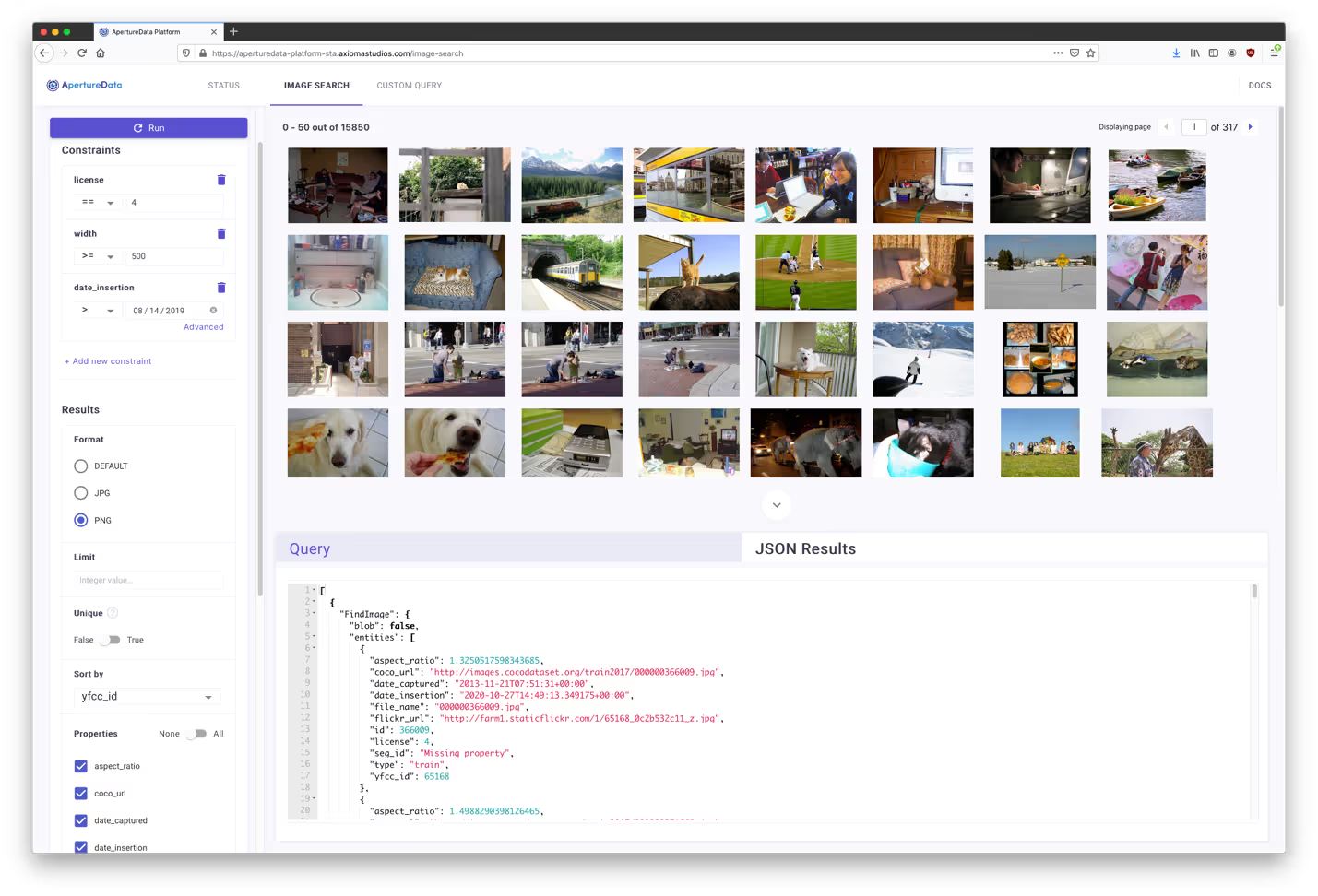
We have made an ApertureDB free trial available through our website , with all the sample code we show here. Simply select the COCO usecase from the dropdown menu, and you will receive an email with instructions on how to access the instance of ApertureDB, pre-populated with the COCO dataset.
Coming up next…
While COCO is a good case to study because of its rich annotations, its size is rather small. We have designed ApertureDB to support a significantly large number of objects while providing the same simple interfaces, without sacrificing performance. We have been using much larger datasets such as the Yahoo Flickr Creative Common 100 million dataset (or YFCC100m for short) both to support real-world customer use cases, and for internal evaluation. We will be releasing this evaluation and more details soon.
Special thanks to Vishakha and Andrei from ApertureData, who helped me shape this article, and to my friends and family that reviewed and annotate countless times.


.png)

.png)



.jpeg)


.png)


